Modeling Social Forces in Microsoft Excel

We know that we are heavily influenced by the opinions and decisions of others, but how can we create a visual representation of that?

Recently, for a problem set in my Behavorial Economics course, we were asked to create a three dimensional model of social forces. The inspiration for this model is derived from Chapter 2 of Weidlich and Haag.

Goals:

• Reproduce figure 2.7
• Demonstrate how our result changes when we change $\kappa$

Clarification

The following words are not my own, but that of my professor, Raymond Hawkins. I believe that he does a really good job explaining this process so I included his outline of the steps for the process below. This is not my work, I only wanted to reproduce it because I was so fascinated with this problem set in particular. I find it quite interesting to share small snippets of my studies; it is quite a privilege.

From Professor Hawkins:

This involves using the master equation with boundary conditions and transition probabilities.

To solve the master equation numerically we will use a discretization known as the Euler approximation:

$P(n$; $t$ + $\Delta$$t$$)$ = $P(n$; $t$$)$ + $\frac{\partial P(n; t)}{\partial t}$$\Delta$$t$

which says that to advance the probability density from time $t$ to time $t$ + $\Delta$$t$ one simply adds to $P(n$; $t$ + $\Delta$$t$$)$ the product $\frac{\partial P(n; t)}{\partial t}$$\Delta$$t$. Since $\frac{\partial P(n; t)}{\partial t}$$\Delta$$t$ is given by the right-hand side of the master equation we have, for a chosen time step $t$, a complete solution: given an initial probability density $P$($n$$;$ $0$), the temporal evolution of $P$($n$$;$ $t$) can be calculated.

The simulation includes:

$\delta$: a preference parameter. A positive value increases the probability that an individual changes from opinion 2 to opinion 1. A negative value increases the probability that an individual changes from opinion 2 to opinion 1.

$\kappa$: an adapatation parameter. A positive value increases the probability of an individual changing to the majority opinion. A negative value decreases the probability of an individual changing to the majority opinion.

$\nu$: a flexibility parameter. Determines the frequency with which (or time scale over which) opinion changes occur.

In cells B3-B9 we are given variables for the simulation. To be clear: there are $2N = 50$ economic agents with psychological parameters $\nu = 1, \kappa = 1$ , and $\delta = 0$. The variables $\kappa_0 = 0.5$ and $\delta_0 = 0$ will be used to specify the probability density $p(n; 0)$ at $t = 0$, and the time step for the simulation is $\Delta t = 0$. This simulates a situation where the economy for $t < 0$ is governed by the variables $\delta_0$ and $\kappa_0$ and for $t \geq0$ by the variables $\delta$ and $\kappa$.

The steps to complete the simulation are as follows:

1. The time axis $t$

We need to specify the time axis to create the graph. The values of the time axis are shown in column A, beginning in cell A25 with $t = 0$ and increasing by $\Delta t = 0.01$ until $t = 6.0$ is reached in cell A625.

2. The configuration axis $n$

We also need to specify the configuration axis for the graph. The values of the configuration axis are shown in row 24, beginning in cell B24 with $n = -N = -25$ and increasing by 1 across row 24 until $n = N = 25$ is reached in cell AZ24.

3. The initial condition

To simulate the temporal evolution of a probability density we need to provide the initial condition, or $p(n; 0)$. There are a variety of ways of getting this of which the simplest is to use the stationary solution:

$\frac{p_{st}(n; 0)}{C}$ $=$ $C$${2N}\choose{N + n}$$\text exp[$$(2$$\delta$$n$ $+$ $\kappa_0$$n$$^{2}/$$N$$]$

where $C = p_{st}(0)\frac{(N!)^2}{(2N)!}$

which is Eq. 2.126 of Weidlich & Haag with the normalization factor $C$. To calculate the initial condition $p(n; 0)$ we start by calculating:

$\frac{p_{st}(n; 0)}{C}$ $=$ ${2N}\choose{N + n}$$\text exp[$$(2$$\delta$$n$ $+$ $\kappa_0$$n$$^{2}/$$N$$]$

since this puts all the $n$ dependence on the right-hand side. These values are shown in row 23 (labeled “Prenormalized”) starting in cell B23 and continuing until cell AZ23: the Excel function COMBIN was used to calculate the binomial coefficient. To calculate the normalization factor $C$, note that summing the left-hand side of

$\frac{p_{st}(n; 0)}{C}$ $=$ ${2N}\choose{N + n}$$\text exp[$$(2$$\delta$$n$ $+$ $\kappa_0$$n$$^{2}/$$N$$]$

yields $\frac{1}{C}$ because $p_{st}(n; 0)$ is a normalized probability density that sums to one. Thus, the sum of the values we have in row 23 is equal to $\frac{1}{C}$ and that sum is shown in cell C22. The normalized initial condition, $p(n; 0)$ shown in cells B25 to AZ25 is obtained by dividing the corresponding cells in row 23 by the value in cell C22.

4. The Temporal evolution

To evolve the probability density through time using the Euler algorithm given in the equation:

$P(n$; $t$ + $\Delta$$t$$)$ = $P(n$; $t$$)$ + $\frac{\partial P(n; t)}{\partial t}$$\Delta$$t$

we need values for $\partial p(n ; t) / \partial t$ which we can get from the master equation in the nearest-neighbor approximation. To this end we need values for $w_{\uparrow}$ and $w_{\downarrow}(n)$. The results of using the expressions on slide 13 of lecture 5 are shown in the screenshot below:

In columns AX-AZ we see in rows 23-25 the calculation described above for $p(n; 0)$ where $23 \leq n \leq 25$. Beginning in column BC we see:

( a ) The values of $w_{\uparrow}(n)$ in row 22.
( b ) The values of $w_{\downarrow}(n)$ in row 23.
( c ) The values of $n$ in row 24 (a repeat of those to the left for convenience.)
( d ) The values of $\partial p(n; t = 0) / \partial t$ in cells BC25 through DA25

The values of $p(n; t = 0.01)$ in cells B26-AZ26 are computed from the values in row 25 using the Euler approximation:

$P(n; t = 0.01) = P(n; t = 0) + \frac{\partial P(n; t = 0)}{\partial t} \times 0.01$ ,

and the corresponding $\partial p(n; t =0.01) / \partial t$ are given in cells BC26-DA26. You can extend this to all $t (0.01 \leq t \leq 6)$ - and thus complete the simulation - by repeating (copying) the calculations in row 26 (columns B to DA) through row 625.

5. Graphing the result

The data in the rectangle defined by the cells from A24 to AZ625 can now be graphed.

End of Professor Hawkins

Analysis

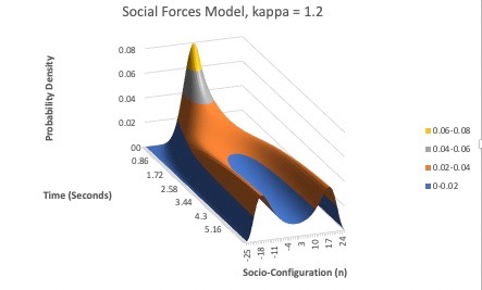
I decided to include a few screenshots of the simulation, for values of $\kappa = 0.5, 1, 1.2$, and $1.5$.

Here is the graph for $\kappa = 0.5$:

For $\kappa = 1$:

For $\kappa =1.2$:

For $\kappa = 1.5$:

Notice how as we increase the value of $\kappa$, the graph becomes more splintered towards either side. For $\kappa = 0.5$, the graph looks very evenly distributed. However, as $\kappa$ increases, we see the graph start to split into two distinct sides. This illustrates how, as $\kappa$ increases, individuals are more likely to change their opinion to that of the majority. A majority of either opinion represents a society that more closely resembles a totalitarian regime, while the opposite is that of a liberal one. I’ll end this short analysis with a quote from the last slide of lecture:

"[a] ‘sound’ banker, alas! is not one who foresees danger andavoids it, but one who, when he is ruined, is ruined in aconventional way along with his fellows, so that no one canreally blame him.”– Keynes 1931.