
Implementing Black Scholes Using Python
Implementing Black Scholes Using Python
#importing all of the necessary modules that we are going to use

import numpy as np
import scipy.stats as si
import sympy as sy
from sympy.stats import Normal, cdf
from sympy import init_printing
init_printing()
The function below creates our black-scholes option pricer.
Function Used to Create Black-Scholes Option Pricer
def black_scholes(S, K, T, r, sigma, option = 'call'):

    #S: spot price
    #K: strike price
    #T: time to maturity
    #r: interest rate
    #sigma: volatility of underlying asset

    d1 = (np.log(S / K) + (r + 0.5 * sigma ** 2) * T) / (sigma * np.sqrt(T))
    d2 = (np.log(S / K) + (r - 0.5 * sigma ** 2) * T) / (sigma * np.sqrt(T))

    if option == 'call':
        call = (S * si.norm.cdf(d1, 0.0, 1.0) - K * np.exp(-r * T) * si.norm.cdf(d2, 0.0, 1.0))
        return call
    if option == 'put':
        put = (K * np.exp(-r * T) * si.norm.cdf(-d2, 0.0, 1.0) - S * si.norm.cdf(-d1, 0.0, 1.0))
        return put
black_scholes(100, 105, 0.5, 0.06, 0.2783, option = 'call')

This cell verifies that our black-scholes option pricer is working properly. The goal was to verify that our pricer spits out the same call price that is given on our lecture slides.
import numpy as np
from datascience import *

# These lines set up graphing capabilities.
import matplotlib
%matplotlib inline
import matplotlib.pyplot as plt
plt.style.use('fivethirtyeight')
import warnings
warnings.simplefilter('ignore', FutureWarning)

from ipywidgets import interact, interactive, fixed, interact_manual
import ipywidgets as widgets
Now, we will build a table and use our option pricer to graph our results.
new_table = Table().with_column("Level of Underlying", np.arange(0,101,10))
new_table.show()
Initial Table
| Level of Underlying |
|---|
| 0 |
| 10 |
| 20 |
| 30 |
| 40 |
| 50 |
| 60 |
| 70 |
| 80 |
| 90 |
| 100 |
#making sure that our Black-Scholes Option pricer works correctly, so we run a sample output and verify with the slide deck from class
#our given inputs are the following:

    #S: spot price
    #K: strike price
    #T: time to maturity
    #r: interest rate
    #sigma: volatility of underlying asset
black_scholes(0.0001, 50, 1, 0.1, 0.39115)

time_to_expiration_of_one_year_array = make_array()
for i in np.arange(0, 101, 10):
    time_to_expiration_of_one_year_array = np.append(time_to_expiration_of_one_year_array, black_scholes(i, 50, 1, 0.1, 0.39115))
<ipython-input-2-76ac2c17deda>:9: RuntimeWarning: divide by zero encountered in log
  d1 = (np.log(S / K) + (r + 0.5 * sigma ** 2) * T) / (sigma * np.sqrt(T))
<ipython-input-2-76ac2c17deda>:10: RuntimeWarning: divide by zero encountered in log
  d2 = (np.log(S / K) + (r - 0.5 * sigma ** 2) * T) / (sigma * np.sqrt(T))
time_to_expiration_of_one_year_array
array([0.00000000e+00, 1.08176967e-04, 7.77138496e-02, 1.07658328e+00,
       4.30794966e+00, 9.99974419e+00, 1.75336194e+01, 2.62035114e+01,
       3.55074908e+01, 4.51478326e+01, 5.49623485e+01])
new_table = new_table.with_column("Time to Expiration of One Year", time_to_expiration_of_one_year_array)
new_table.show()
Table of Time to Expiration of One Year
| Level of Underlying | Time to Expiration of One Year |
|---|---|
| 0 | 0 |
| 10 | 0.000108177 |
| 20 | 0.0777138 |
| 30 | 1.07658 |
| 40 | 4.30795 |
| 50 | 9.99974 |
| 60 | 17.5336 |
| 70 | 26.2035 |
| 80 | 35.5075 |
| 90 | 45.1478 |
| 100 | 54.9623 |
no_time_to_expiration_array = make_array()
for i in np.arange(0, 101, 10):
    no_time_to_expiration_array = np.append(no_time_to_expiration_array, black_scholes(i, 50, 0.0000001, 0.1, 0.39115))
<ipython-input-2-76ac2c17deda>:9: RuntimeWarning: divide by zero encountered in log
  d1 = (np.log(S / K) + (r + 0.5 * sigma ** 2) * T) / (sigma * np.sqrt(T))
<ipython-input-2-76ac2c17deda>:10: RuntimeWarning: divide by zero encountered in log
  d2 = (np.log(S / K) + (r - 0.5 * sigma ** 2) * T) / (sigma * np.sqrt(T))
no_time_to_expiration_array
array([0.00000000e+00, 0.00000000e+00, 0.00000000e+00, 0.00000000e+00,
       0.00000000e+00, 2.46755821e-03, 1.00000005e+01, 2.00000005e+01,
       3.00000005e+01, 4.00000005e+01, 5.00000005e+01])
new_table = new_table.with_column("Time to Expiration of None", no_time_to_expiration_array )
new_table.show()
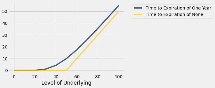
Graph of Time to Expiration of Both One and Zero Years
| Level of Underlying | Time to Expiration of One Year | Time to Expiration of None |
|---|---|---|
| 0 | 0 | 0 |
| 10 | 0.000108177 | 0 |
| 20 | 0.0777138 | 0 |
| 30 | 1.07658 | 0 |
| 40 | 4.30795 | 0 |
| 50 | 9.99974 | 0.00246756 |
| 60 | 17.5336 | 10 |
| 70 | 26.2035 | 20 |
| 80 | 35.5075 | 30 |
| 90 | 45.1478 | 40 |
| 100 | 54.9623 | 50 |
new_table.plot("Level of Underlying")
three_year_array = make_array()
for i in np.arange(0, 101, 10):
    three_year_array = np.append(three_year_array, black_scholes(i, 50, 3, 0.1, 0.39115))
<ipython-input-2-76ac2c17deda>:9: RuntimeWarning: divide by zero encountered in log
  d1 = (np.log(S / K) + (r + 0.5 * sigma ** 2) * T) / (sigma * np.sqrt(T))
<ipython-input-2-76ac2c17deda>:10: RuntimeWarning: divide by zero encountered in log
  d2 = (np.log(S / K) + (r - 0.5 * sigma ** 2) * T) / (sigma * np.sqrt(T))
three_year_array
array([ 0.        ,  0.12653854,  1.75641839,  5.77813145, 11.7582735 ,
       19.0826488 , 27.28807781, 36.06767126, 45.22466791, 54.63318365,
       64.21192494])
new_table = new_table.with_column("Time to Expiration of Three Years", three_year_array)
new_table.show()
Graph of All Three Times to Expiration
| Level of Underlying | Time to Expiration of One Year | Time to Expiration of None | Time to Expiration of Three Years |
|---|---|---|---|
| 0 | 0 | 0 | 0 |
| 10 | 0.000108177 | 0 | 0.126539 |
| 20 | 0.0777138 | 0 | 1.75642 |
| 30 | 1.07658 | 0 | 5.77813 |
| 40 | 4.30795 | 0 | 11.7583 |
| 50 | 9.99974 | 0.00246756 | 19.0826 |
| 60 | 17.5336 | 10 | 27.2881 |
| 70 | 26.2035 | 20 | 36.0677 |
| 80 | 35.5075 | 30 | 45.2247 |
| 90 | 45.1478 | 40 | 54.6332 |
| 100 | 54.9623 | 50 | 64.2119 |
new_table.plot("Level of Underlying")
plt.xlabel('Level of Underlying (Arbitrary) ')
plt.ylabel('Price (Arbitrary) ')
Text(0, 0.5, 'Price (Arbitrary) ')
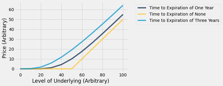
Final Graph
This is the final graph that we were supposed to replicate from our lecture slides. Mission accomplished! We can see that, at option expiration, the graph of the underlying and price has the sharp, rigid slope that we were looking for. In contrast, the other two curves are just that, curved. That is exactly what we would expect with the given inputs.
def black_scholes(S, K, T, r, sigma, option = 'call'):

    #S: spot price
    #K: strike price
    #T: time to maturity
    #r: interest rate
    #sigma: volatility of underlying asset

    d1 = (np.log(S / K) + (r + 0.5 * sigma ** 2) * T) / (sigma * np.sqrt(T))
    d2 = (np.log(S / K) + (r - 0.5 * sigma ** 2) * T) / (sigma * np.sqrt(T))

    if option == 'call':
        call = (S * si.norm.cdf(d1, 0.0, 1.0) - K * np.exp(-r * T) * si.norm.cdf(d2, 0.0, 1.0))
        return call
    if option == 'put':
        put = (K * np.exp(-r * T) * si.norm.cdf(-d2, 0.0, 1.0) - S * si.norm.cdf(-d1, 0.0, 1.0))
        return put
black_scholes(100, 105, 0.5, 0.06, 0.2783, option = 'call')

black_scholes(85, 105, 0.5, 0.06, 0.2783, option = 'call')

black_scholes(85, 105, 0.5, 0.06, 0.2783, option = 'put')

black_scholes(100, 105, 0.5, 0.06, 0.5, option = 'call')

Conclusion
These last few lines were further verification of our option pricer. We tested different volatilities and spot prices, and also looked at the different prices associated with calls and puts.