Data Science Analysis of Running Form

Analyzing the Correlation Between Running Stride Length and Average Pace Per Mile

from datascience import *
%matplotlib inline
import matplotlib.pyplot as plots
plots.style.use('fivethirtyeight')
import numpy as np

Importing the Data

The data generating process was as follows: I went on my run. Once I finished my run, I saved it. I uploaded the run to my iPhone via bluetooth. Once the running data uploaded, I exported a CSV file of the data to my computer.

Here is a link to the google sheets version of the data. For reference, the watch I used to collect this data is the COROS Pace 2.

As a side note, this statistical analysis only takes into account one run. In the future I plan to run a more comprehensive analysis because it is essential to have a variety of data to truly prove a statistical relationship. However, this is a good jumping-off point.

The following running data is from an 18 mile long run. I started at 6:39 mile pace and closed in 5:27 for the last mile. As it was progressive, I chose to analyze the linear relationship between stride length as running pace increases. For the actual analysis, I used the column that contains minutes per kilometer rather than minutes per mile. We are also, for the purpose of this project, holding constant external factors such as elevation gain per mile, heart rate, and prior muscle fatigue.

progressive_longrun_data = Table.read_table("ProgressiveLongRun.csv")
progressive_cleaned = progressive_longrun_data.take(np.arange(0,18,1))
progressive_cleaned.show()

Split	Time	Moving Time	Distance	Elevation Gain	Elev Loss	Avg Pace	Avg Moving Pace	Best Pace	Avg Run Cadence	Max Run Cadence	Avg Stride Length	Avg HR	Max HR	Avg Temperature	Calories
1	0:06:39	0:06:39	1.61	0	31	0:04:08	0:04:05	0:03:39	82	84	148	128	147	24	48
2	0:06:33	0:06:33	1.61	6	30	0:04:04	0:04:03	0:03:46	82	83	150	141	145	22	63
3	0:06:33	0:06:33	1.61	27	21	0:04:04	0:04:08	0:03:47	83	86	149	149	154	20	59
4	0:06:31	0:06:31	1.61	16	31	0:04:03	0:04:04	0:03:54	82	85	150	151	153	21	70
5	0:06:33	0:06:33	1.61	56	15	0:04:04	0:04:06	0:03:14	84	89	147	148	156	21	58
6	0:06:31	0:06:31	1.61	5	31	0:04:03	0:04:02	0:03:52	82	85	150	155	165	23	72
7	0:06:29	0:06:29	1.61	49	0	0:04:02	0:04:01	0:03:51	84	87	148	167	172	23	70
8	0:06:31	0:06:27	1.61	34	4	0:04:00	0:04:01	0:03:47	84	86	148	165	173	24	68
9	0:06:27	0:06:27	1.61	7	29	0:04:00	0:04:01	0:03:48	83	85	151	159	167	25	65
10	0:06:21	0:06:21	1.61	0	34	0:03:57	0:03:57	0:03:52	83	84	154	162	170	25	78
11	0:06:15	0:06:15	1.61	0	35	0:03:53	0:03:53	0:03:38	83	85	155	165	169	25	69
12	0:06:12	0:06:12	1.61	34	24	0:03:51	0:03:53	0:03:37	84	88	154	165	170	24	68
13	0:06:05	0:06:05	1.61	15	32	0:03:47	0:03:49	0:03:28	84	89	157	159	167	24	66
14	0:05:55	0:05:55	1.61	46	17	0:03:41	0:03:41	0:02:46	86	90	159	164	176	23	67
15	0:05:51	0:05:51	1.61	17	30	0:03:38	0:03:39	0:03:23	84	86	163	168	173	24	71
16	0:05:46	0:05:46	1.61	48	1	0:03:35	0:03:38	0:03:29	87	89	162	171	177	23	72
17	0:05:39	0:05:39	1.61	38	5	0:03:31	0:03:32	0:03:24	86	89	165	172	179	23	61
18	0:05:27	0:05:27	1.61	9	22	0:03:23	0:03:21	0:02:53	87	91	169	173	180	24	74

Initial Visualization of the Data

We want to look at an initial visualization of the data so that we can see if there are any obvious patterns. Upon initial inspection, there looks to be good possibility for a linear relationship between average running pace and average stride length.

progressive_cleaned.scatter("Avg Pace", "Avg Stride Length")
plots.xlabel("Average Running Pace (Minutes per Kilometer)")
plots.ylabel("Average Stride Length (Centimeters)")

Text(0, 0.5, 'Average Stride Length (Centimeters)')

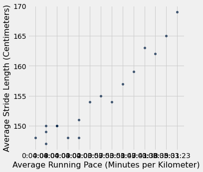
In the initial visualization of the data, it becomes apparent that the minutes and second display on the x axis isn’t very elegant. Consequently, I spent the following lines of code converting the average pace per kilometer from a minutes and seconds version to purely seconds form.

import datetime

string_version = [str(i) for i in progressive_cleaned.column("Avg Pace")]
#modifying the running time in minutes per kilometer from elements in a numpy array to individual strings

updated_list = []
#creating an empty list that we can append the datetime version of the strings to
for i in string_version:
    date_time_version = datetime.datetime.strptime(i, "%H:%M:%S")
    updated_list.append(date_time_version)

updated_list

final_list = []
#the final list for which we are going to append the time in seconds per kilometer
for i in updated_list:
    a_timedelta = i - datetime.datetime(1900, 1, 1)
    seconds = a_timedelta.total_seconds()
    final_list.append(int(seconds))

running_pace_vs_stride_length = Table().with_column("Average Running Pace", final_list).with_column("Average Stride Length", progressive_cleaned.column("Avg Stride Length"))

running_pace_vs_stride_length.show()

Average Running Pace	Average Stride Length
248	148
244	150
244	149
243	150
244	147
243	150
242	148
240	148
240	151
237	154
233	155
231	154
227	157
221	159
218	163
215	162
211	165
203	169

running_pace_vs_stride_length.scatter("Average Running Pace", "Average Stride Length")
plots.xlabel("Average Running Pace (Seconds per Kilometer)")
plots.ylabel("Average Stride Length (Centimeters)")

Text(0, 0.5, 'Average Stride Length (Centimeters)')

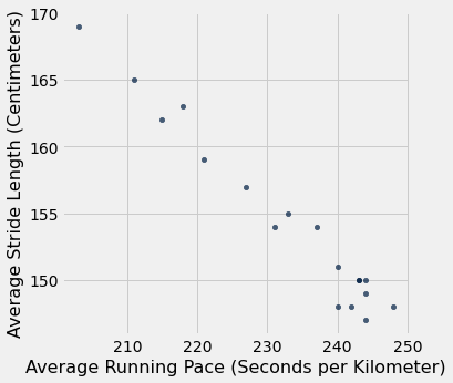
Now we have cleaned the data, dropped the unnecessary parts, and have a simple visualization of what we are going to look at in further detail. We have a two column table containing what we would like to analyze for this particular moment. Time for some statistical testing.

# Creating some functions that we will use to analyze the data.
#We need standard units so that we can run our correlation function.

def standard_units(x):
    """ Converts an array x to standard units """
    return (x - np.mean(x)) / np.std(x)

def correlation(t, x, y):
    """ Computes correlation: t is a table, and x and y are column names """
    x_su = standard_units(t.column(x))
    y_su = standard_units(t.column(y))
    return np.mean(x_su * y_su)

#generating the correlation coefficient
correlation(running_pace_vs_stride_length, "Average Running Pace", "Average Stride Length")

-0.9819409345425044

Wow! We generated a correlation coefficient of -0.98, which means there is almost an exactly proportionate decrease in stride length for an increase in the amount of seconds it take to complete each kilometer! However, a correlation coefficient alone is not enough. We need to also look at a linear regression line and plot the residuals.

#our slope and intercept functions
def slope(t, x, y):
    """ Computes the slope of the regression line, like correlation above """
    r = correlation(t, x, y)
    y_sd = np.std(t.column(y))
    x_sd = np.std(t.column(x))
    return r * y_sd / x_sd

def intercept(t, x, y):
    """ Computes the intercept of the regression line, like slope above """
    x_mean = np.mean(t.column(x))
    y_mean = np.mean(t.column(y))
    return y_mean - slope(t, x, y)*x_mean

slope_for_regression_line = slope(running_pace_vs_stride_length, "Average Running Pace", "Average Stride Length")
slope_for_regression_line

-0.48736086175942556

intercept_for_regression_line = intercept(running_pace_vs_stride_length, "Average Running Pace", "Average Stride Length")
intercept_for_regression_line

267.67321364452425

#generating the predicted stride length from running pace and adding that to the table
predictions = slope_for_regression_line * running_pace_vs_stride_length.column("Average Running Pace") + intercept_for_regression_line

predictions

array([146.80771993, 148.75716338, 148.75716338, 149.24452424,
       148.75716338, 149.24452424, 149.7318851 , 150.70660682,
       150.70660682, 152.16868941, 154.11813285, 155.09285458,
       157.04229803, 159.9664632 , 161.42854578, 162.89062837,
       164.84007181, 168.73895871])

run_with_predictions = running_pace_vs_stride_length.with_column("Predicted Stride Length", predictions)

run_with_errors = run_with_predictions.with_column("Error", run_with_predictions.column("Average Stride Length") - run_with_predictions.column("Predicted Stride Length"))

run_with_errors.show()

Average Running Pace	Average Stride Length	Predicted Stride Length	Error
248	148	146.808	1.19228
244	150	148.757	1.24284
244	149	148.757	0.242837
243	150	149.245	0.755476
244	147	148.757	-1.75716
243	150	149.245	0.755476
242	148	149.732	-1.73189
240	148	150.707	-2.70661
240	151	150.707	0.293393
237	154	152.169	1.83131
233	155	154.118	0.881867
231	154	155.093	-1.09285
227	157	157.042	-0.042298
221	159	159.966	-0.966463
218	163	161.429	1.57145
215	162	162.891	-0.890628
211	165	164.84	0.159928
203	169	168.739	0.261041

root_mean_squared_error = np.mean(run_with_errors.column("Error") ** 2) ** 0.5

root_mean_squared_error

1.2311567965332846

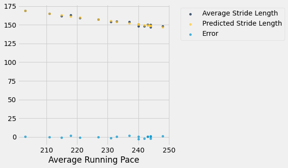
run_with_errors.scatter("Average Running Pace")

Taking A Closer Look at the Residuals

From that plot, we can tell that the trend in the residuals looks good. The aim of any linear regression estimate is to generate residuals that appear as white noise. However, the plot is a little bit zoomed out. Let’s manipulate the x and y axis to generate a closer look at the residuals.

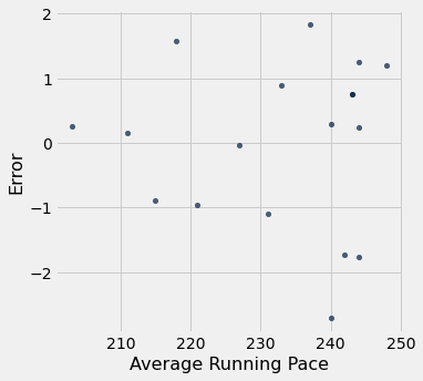
run_with_errors.scatter("Average Running Pace", "Error")

mean_stride_length = np.mean(run_with_errors.column("Average Stride Length"))
mean_stride_length

154.38888888888889

maximum_error = max(abs(run_with_errors.column("Error")))
maximum_error

2.706606822262131

2 / 154.38

0.012955045990413267

root_mean_squared_error

1.2311567965332846

root_mean_squared_error / mean_stride_length

0.007974387311118792

With this zoomed in look, we can tell that most of our errors hover around the range +- 2. This means that our usual error is around 2 centimeters. That’s not a bad error. Given the mean stride length of 154, the predicted percentage of stride length that we will be off by is about 1.3 percent. That’s a darn good estimate. If we take into consideration the RMSE of 1.23, we take 1.23 / 154.38 and get a result of 0.007, which is 0.7 percent.

Conclusion

From analysis of the errors, and correlation coefficient of -0.98, we can conclude that linear prediction is a good indicator for calculating my stride length, given a running pace between 200 and 300 seconds per kilometer.

Back to Top